Introduction to the Moltres Input File Syntax

Model Geometry

The figure below shows the domain for the 2-D MSRE model. It is a 72.2 cm by 165 cm rectangle that is axisymmetric about the left boundary. The domain consists of 14 fuel channels, alternating with 14 solid graphite moderator regions, represented in the figure by gray and red rectangles, respectively.

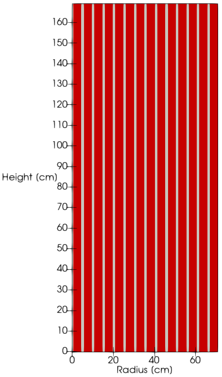
Figure 1: 2-D axisymmetric model of the MSRE

File Format

Moltres is built on top of the MOOSE framework, and the input file uses the "hierarchical input text format" (hit) input format adopted by MOOSE. A brief description of the input syntax is presented here. This is a relatively simple file format that uses [names in brackets] to mark the start of input blocks. Empty brackets [] are used to indicate the end of a block. Note that block names and parameter names are generally case sensitive in the input file. In addition, in Moltres/MOOSE input files, the # symbol is used to mark the start of a comment. Comments may start anywhere on a line.

Substitution Variables

Root level variables can be used as substitution variables throughout the document by using the syntax ${varname}. Starting at the top of the input file, the following substitution variables are defined:

flow_velocity=17.55  # cm/s

flow_velocity is used to set the upward flow velocity of the fuel/molten salt in this model. Comments can be added after the # character for inline documentation.

You may set the flow velocity to zero to obtain the multiplication factor of this system without delayed neutron precursor (DNP) drift. Note that this input file does not model the looping of DNPs back into the core after flowing through out-of-core components. Therefore, all DNPs flowing out of the core are considered lost.

GlobalParams Block

Following the substitution variable definitions, we have the GlobalParams block:

[GlobalParams]
  num_groups = 2
  num_precursor_groups = 6
  use_exp_form = false
  group_fluxes = 'group1 group2'
  temperature = temp
  sss2_input = true
  pre_concs = 'pre1 pre2 pre3 pre4 pre5 pre6'
  account_delayed = true
[]

In GlobalParams, parameters like num_groups can be globally set to a value. Consequently any class (e.g. the kernel class GroupDiffusion) that has the parameter num_groups will read in a value of 2 unless it is overridden locally in its input block. It should be noted that the GlobalParams block and any other MOOSE input block can be placed anywhere in the input file. At execution time each block will be read when it is needed. Below is a description of the parameters included in the GlobalParams section:

• num_groups: The number of energy groups for neutron diffusion

• num_precursor_groups: The number of delayed neutron precursor groups

• use_exp_form: Whether the actual neutron/precursor fluxes/concentrations should be represented by or where is the actual variable value

• group_fluxes: The names of the neutron group fluxes

• temperature: The name of the temperature variable. Some of the kernel or boundary condition variables require an input named temperature which specifies the variable used to represent temperature. The variable temp will be specified below in the [Variables] block.

• sss2_input: True if the macroscopic group constants were generated by Serpent 2 or OpenMC. False otherwise

• pre_concs: The names of the precursor concentration variables

• account_delayed: Whether to account for delayed neutron production. Modifies the neutron source term

Mesh Block

Next in our input file we have the Mesh block. The two most commonly used Mesh types are FileMesh and GeneratedMesh. The Mesh input block by default assumes type FileMesh and takes a parameter argument file = <mesh_file_name>.

[Mesh]
  coord_type = RZ
  [mesh]
    type = FileMeshGenerator
    file = 'mesh.e'
  []
[]

We use coord_type to indicate to Moltres that this is a 2-D axisymmetric problem. By default, it takes a xy-coordinate mesh and considers the y-axis (x=0) to be the axis of symmetry.

MOOSE has an extensive MeshGenerators system for generating simple meshes or making simple edits. We refer the reader here for more information about the system. The mesh.i file uses this system to generate the mesh for the parallel channel structure of the 2-D MSRE model. The 'mesh.e' file for this tutorial can be generated by running the following command:

../../moltres-opt -i mesh.i --mesh-only mesh.e

Many MOOSE users generate more complex meshes using Cubit/Trelis. For national lab employees this software is free; however, academic or industry users must pay. Consequently, many of Moltres meshes to date have been generated using MeshGenerators or the open-source software gmsh. Gmsh binaries for Windows, Mac, and Linux as well as source code can be downloaded here. Ubuntu users may also install Gmsh using sudo apt-get install gmsh. We will not go into the details of using Gmsh but the interested user should peruse its documentation. There are many example Gmsh input files in the Moltres repository (denoted by the .geo extension). To generate a mesh for use with Moltres, a typical bash command is gmsh -2 -o file_name.msh file_name.geo where 2 should be replaced with the dimension of the mesh, the argument following -o is the name of the output .msh file, and the last argument is the input .geo file.

Problem Block

The Problem block is used to indicate the type of problem we are solving. MOOSE automatically identifies which problem class is suitable for your simulation type (e.g., FEProblem or EigenProblem). However, for this particular input file, we want to set the bx_norm parameter for determining the eigenvalue estimate during each iteration of the eigensolver. Therefore, this input file requires us to indicate the problem type and the bx_norm parameter.

[Problem]
  type = EigenProblem
  bx_norm = bnorm
[]

Variables Block

The Variables block is used to indicate the primary solution variables, or equivalently, to indicate the number of partial differential equations (PDEs) that will be defined in the Kernels and BCs blocks. For this model, the group1 and group2 neutron fluxes are the system variables that are being solved for by the PDEs. In the Kernels and BCs blocks described below, each kernel and BC term must be associated with one primary variable from the Variables list below to indicate which PDE the term is included in.

[Variables]
  [group1]
    order = FIRST
    family = LAGRANGE
  []
  [group2]
    order = FIRST
    family = LAGRANGE
  []
[]

Sub-blocks are initialized with [<object_name>] and closed with []. The [group1] sub-block creates a MooseVariable object with the name group1. The parameters purpose of the parameter is as follows:

• family describes the shape function type used to form the approximate finite element solution.

• order denotes the polynomial order of the shape functions.

• initial_condition is an optional parameter that can be used to set a spatially uniform initial value for the variable.

• scaling is another optional parameter that can be used to scale the residual of the corresponding variable; this is usually done when different variables have residuals of different orders of magnitude.

Precursors Block

Whereas all the other blocks that have been introduced are standard MOOSE blocks, Precursors is a custom input file block unique to Moltres. The Precursors action sets up the delayed neutron precursor concentration equations:

The precursor variables, kernels, and boundary conditions necessary for solving the precursor governing equations are all instantiated by the Precursors action. Six precursor groups (symbolized by the index i in the equation above) are modeled, as specified via the num_precursor_groups in the GlobalParams block. is the number of neutron flux energy groups, and is the index associated with the energy groups. For this problem two energy groups are modeled, with the equations configured explicitly in the Kernels and BCs blocks documented after this section.

[Precursors]
  [./pres]
    var_name_base = pre
    family = MONOMIAL
    order = CONSTANT
    block = 'fuel'
    outlet_boundaries = 'fuel_top'
    constant_velocity_values = true
    u_def = 0
    v_def = ${flow_velocity}
    w_def = 0
    nt_exp_form = false
    loop_precursors = false
    transient = false
    eigen = true
  [../]
[]

Parameter descriptions:

• var_name_base: The prefix for the precursor variable names. Name suffixes are numbers, e.g. pre1, pre2, ...

• block: This is a parameter ubiquitous to many MOOSE classes such as kernels and materials. By specifying a value for block the user is asking that in this case, precursors and their associated governing equations only be solved for in the fuel mesh subdomains

• outlet_boundaries: The mesh boundaries from which the precursors flow out

• u_def, v_def, w_def: The x, y, and z components of velocity, or in the case of an RZ simulation, u_def is the r velocity component, v_def is the z-component, and w_def has no meaning

• nt_exp_form: Whether the neutron group fluxes have their concentrations in an exponential form. If use_exp_form is false in the GlobalParams block, this should also be false

• loop_precursors: Whether the DNPs are looped back into the core through the flow inlet

• transient: Whether this is a transient or time-independent simulation

• eigen: Whether this is an eigenvalue problem

Kernels Block

The Kernels block is used to construct PDEs that are included in the system of equations that are solved. Each PDE has a primary variable that is being solved for, and the list of variables being solved for is defined in the Variables block shown above. There is an additional PDE solved as part of the system of PDEs for each variable defined in the Variables section. In this case, three solution variables were defined in the variable section:

• The group1 fast group neutron flux.

• The group2 thermal group neutron flux.

Note that additional precursor variables are automatically defined by the Precursors block.

The Kernels section defines a set of "Kernels", where a "Kernel" represents a single term included in a PDE. A PDE is constructed by specifying the set of terms (or Kernels) that will be included in the PDE in the Kernels block, and by specifying which PDE the kernel is associated with. This is done by indicating which of the above three variables the kernel is associated with (i.e., group1 or group2).

Thus, each entry in the Kernels block specifies a term to include in one of PDEs that are solved. The type = <kernel type> parameter associated with a kernel entry identifies the term (or Kernel) that will be included in the PDE, and the variable = <primary variable> value indicates the primary solution variable (from the Variables block) associated with the term, or equivalently which PDE the term will be included in. MOOSE provides several standard kernels that can be included in a PDE. Moltres defines an additional set of kernels that are useful in modeling neutron flux and associated phenomenon in molten salt reactors. The mathematical form of each Moltres kernel can be found its corresponding documentation webpage on Moltres Syntax.

Kernels can be optionally restricted to specific subdomains within the model by setting block = <subdomain_names>. Note that this implies that the form of the equation that is solved may differ in different mesh regions. The equations that are modeled are represented below, followed by the input required to construct these equations. In the group1 and group2 neutron flux equations below and in the input that follows, notice that the fission kernel (CoupledFissionKernel) is only included in the fuel region ('0'), and is not included in the moderator region ('1') since there is no fuel in the moderator region. Also, the DelayedNeutronSource kernel, which contributes neutrons from the precursor group equations, is only included as part of the group1 or fast group equation.

Neutron Diffusion Equation for the k-Eigenvalue Problem with group1 and group2 Variables (g = 1 or 2)

The extra_vector_tags = eigen parameter indicates all kernels to be scaled by the eigenvalue in this eigenvalue problem. This parameter is omitted for non-eigenvalue problems discussed in the other tutorial problems.

[Kernels]
  #---------------------------------------------------------------------
  # Group 1 Neutronics
  #---------------------------------------------------------------------
  [sigma_r_group1]
    type = SigmaR
    variable = group1
    group_number = 1
  []
  [diff_group1]
    type = GroupDiffusion
    variable = group1
    group_number = 1
  []
  [inscatter_group1]
    type = InScatter
    variable = group1
    group_number = 1
  []
  [fission_source_group1]
    type = CoupledFissionKernel
    variable = group1
    group_number = 1
    block = '0'
    extra_vector_tags = 'eigen'
  []
  [delayed_group1]
    type = DelayedNeutronSource
    variable = group1
    block = '0'
    group_number = 1
  []

  #---------------------------------------------------------------------
  # Group 2 Neutronics
  #---------------------------------------------------------------------
  [sigma_r_group2]
    type = SigmaR
    variable = group2
    group_number = 2
  []
  [diff_group2]
    type = GroupDiffusion
    variable = group2
    group_number = 2
  []
  [fission_source_group2]
    type = CoupledFissionKernel
    variable = group2
    group_number = 2
    block = '0'
    extra_vector_tags = 'eigen'
  []
  [inscatter_group2]
    type = InScatter
    variable = group2
    group_number = 2
  []
[]

BCs Block

The BCs block is very similar to the Kernels block except the boundary = <boundary_names> parameter must be specified to indicate where the boundary conditions should be applied. Documentation for the BCs can be also found on the Moltres Syntax page.

[BCs]
  [vacuum_group1]
    type = VacuumConcBC
    boundary = 'fuel_bottom fuel_top mod_bottom mod_top right'
    variable = group1
  []
  [vacuum_group2]
    type = VacuumConcBC
    boundary = 'fuel_bottom fuel_top mod_bottom mod_top right'
    variable = group2
  []
[]

Materials Block

In the Materials block, we specify materials that live on a mesh subdomain. Any given subdomain can have as many material definitions as desired, so long as a property is not multiply defined. We use MoltresJsonMaterial here which is used to parse the JSON-based group constant data file.

[Materials]
  [fuel]
    type = MoltresJsonMaterial
    block = '0'
    base_file = 'xsdata.json'
    material_key = 'fuel'
    interp_type = LINEAR
    prop_names =''
    prop_values = ''
  []
  [graphite]
    type = MoltresJsonMaterial
    block = '1'
    base_file = 'xsdata.json'
    material_key = 'graphite'
    interp_type = LINEAR
    prop_names =''
    prop_values = ''
  []
[]

Materials within the Materials block support the following parameters:

• base_file: The relative/absolute path and name of the JSON file containing the macroscopic group constants that define neutron interactions in this material.

• material_key: The name of the material in the JSON file that corresponds to this Material object.

• interp_type: The type of fitting/interpolation to be carried out on the temperature grid. Options are:

  • spline: Cubic spline interpolation

  • linear: Linear spline interpolation

  • monotone_cubic: Monotone cubic interpolation

  • none: Only should be used when single values for constants are supplied at a single temperature

• prop_names, prop_values: name-value pairs used to define material property values from the input file. For example, the density , thermal conductivity , and the specific heat capacity may be defined for simulations involving a temperature variable.

Executioner and Preconditioning Blocks

The Executioner and Preconditioning blocks are essential for setting the method used to solve the system of non-linear equations created by finite element discretization of our molten salt reactor governing equations. Executioner and Preconditioning documentation can be found here and here respectively. You may also refer to our guide for basic instructions.

[Executioner]
  type = Eigenvalue
  initial_eigenvalue = 1
  solve_type = 'PJFNK'
  petsc_options = '-snes_converged_reason -ksp_converged_reason -snes_linesearch_monitor'
  petsc_options_iname = '-pc_type -pc_hypre_type'
  petsc_options_value = 'hypre boomeramg'

  automatic_scaling = true
  compute_scaling_once = false
  resid_vs_jac_scaling_param = 0.1

  line_search = none
[]

Postprocessors Block

A PostProcessor computes a single scalar value during the simulations. General postprocessor documentation can be found here.

k_eff retrieves the real part of the computed eigenvalue which is taken to be the multiplication factor. The bnorm, tot_fissions, and powernorm postprocessor objects calculate the total number of fission neutrons, fission interactions, and fission heat, respectively. The bnorm parameter is required by the Eigenvalue executioner as an estimate for in each iteration. The other two may be used to normalize the flux solution at the end of the calculation through the normalization and normal_factor parameters in the Executioner block. The rest of the postprocessors calculate the integral sum, diff, or maximum values of the group1 and group2 flux variables.

[Postprocessors]
  [k_eff]
    type = VectorPostprocessorComponent
    index = 0
    vectorpostprocessor = k_vpp
    vector_name = eigen_values_real
  []
  [bnorm]
    type = ElmIntegTotFissNtsPostprocessor
    execute_on = linear
  []
  [tot_fissions]
    type = ElmIntegTotFissPostprocessor
    execute_on = linear
  []
  [powernorm]
    type = ElmIntegTotFissHeatPostprocessor
    execute_on = linear
  []
  [group1norm]
    type = ElementIntegralVariablePostprocessor
    variable = group1
    execute_on = linear
  []
  [group1max]
    type = NodalExtremeValue
    value_type = max
    variable = group1
    execute_on = timestep_end
  []
  [group1diff]
    type = ElementL2Diff
    variable = group1
    execute_on = 'linear timestep_end'
  []
  [group2norm]
    type = ElementIntegralVariablePostprocessor
    variable = group2
    execute_on = linear
  []
  [group2max]
    type = NodalExtremeValue
    value_type = max
    variable = group2
    execute_on = timestep_end
  []
  [group2diff]
    type = ElementL2Diff
    variable = group2
    execute_on = 'linear timestep_end'
  []
[]

Outputs Block

In the Outputs block, we can control the settings for various data output formats. Outputs documentation is here. In this input file, the Exodus and CSV output formats are enabled with default settings associated with each output type. print_graph prints various computational performance information in the console (e.g., time taken in each section of the simulation). print_linear_residuals prints all linear residual values during the simulation, which may be desired when running test runs.

[Outputs]
  print_graph = true
  print_linear_residuals = true
  [exodus]
    type = Exodus
  []
  [csv]
    type = CSV
  []
[]

Debug Block

This parameter tells Moltres to print the variable residual norms during the non-linear solve. Residual information is useful for debugging convergence issues by identifying which variable is exhibiting slow or no convergence behavior.

[Debug]
  show_var_residual_norms = true
[]